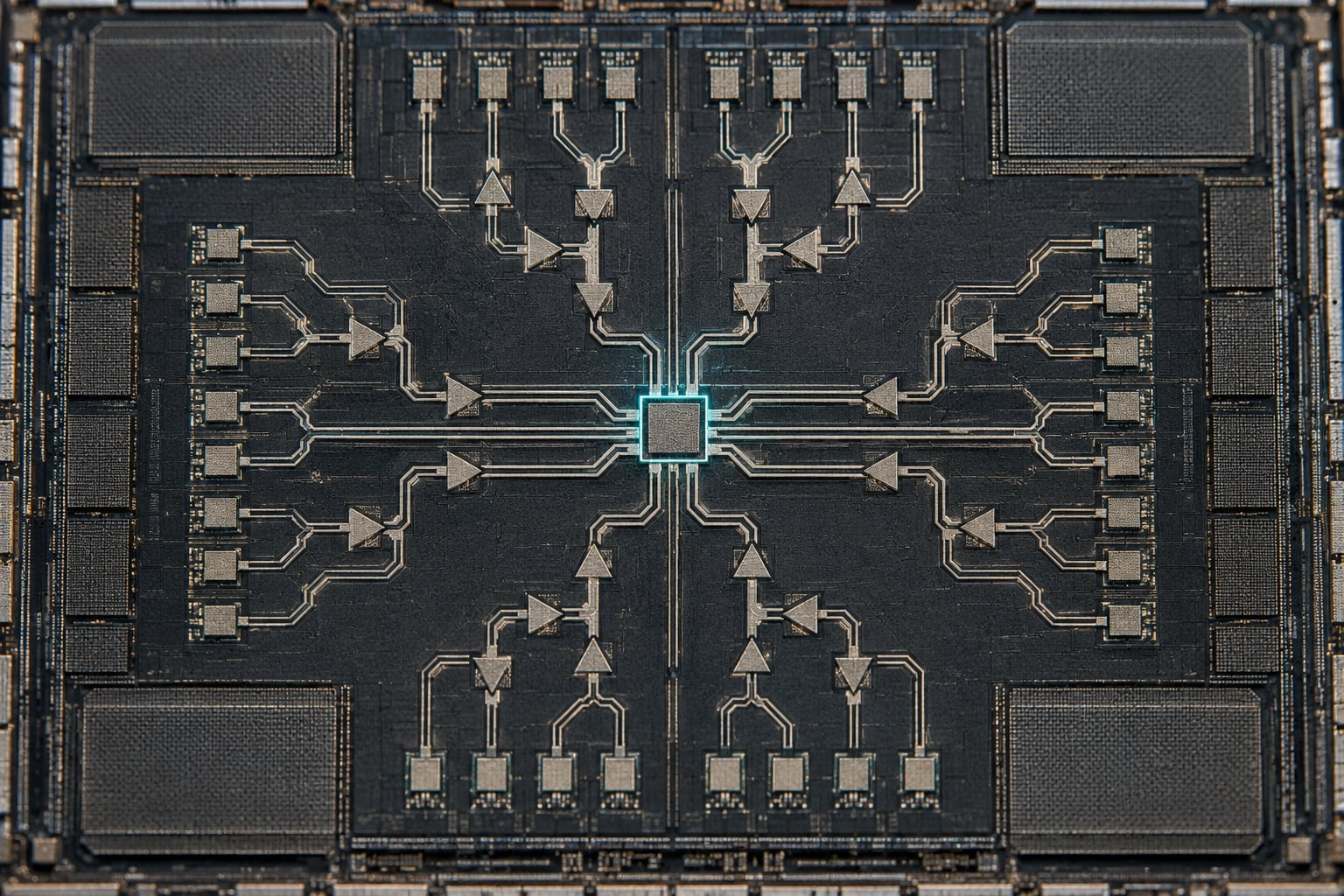
Clock Tree Synthesis Explained: A Practical Guide 2026

Clock tree synthesis explained in one sentence: it is the physical design step where an EDA tool inserts clock buffers and inverters between a design’s clock source and the clock pins of its sequential cells, building a balanced tree-shaped network that delivers the clock to every register at nearly the same arrival time. The buffer tree drives every flip-flop while balancing insertion delay and clock skew.

Before the tool builds anything, it reads the SDC clock constraints, finds every clock sink pin in the placed netlist, and then propagates outward from the clock root. What comes out the other side is a routed network of clock cells with a reported skew, a reported insertion latency, and a power bill that appears in every later power report.

This guide walks through what the tree looks like, why balance matters, which algorithms commercial tools actually run, and how to debug a tree that did not come out the way you expected.

Table of Contents

• What Is Clock Tree Synthesis?
• The anatomy of a clock tree
• Why Does a Clock Tree Need to Be Balanced?
• How Does Clock Tree Synthesis Build the Network?
• Which topologies the algorithms use
• What Happens During Clock Tree Synthesis?
• How Do CTS and STA Work Together?
• How Does CTS Affect Power, Area, and Routing?
• What Problems Can Cause a Bad Clock Tree?
• How Do You Verify and Fix a Clock Tree?
• Clock Tree Synthesis Explained: Key Terms and Design Choices
• Frequently Asked Questions
• What is the difference between clock skew and clock latency?
• When should CTS be performed in the physical design flow?
• Is CTS performed before or after clock gating?
• What is useful skew in clock tree synthesis?
• How do I know whether my clock tree is balanced?
• Why can CTS fix timing but increase clock power?
• Conclusion

What Is Clock Tree Synthesis?

Clock tree synthesis (CTS) is the step that turns a single clock port into a distribution network. It is also called clock tree building, clock tree balancing or, less formally, clock routing.

The tree is a logic structure plus a physical structure. Logically you have one clock net leaving the source and arriving at many sink pins. Physically the tool has inserted buffers, inverters and clock gating cells in between, and it has placed them so the delay from source to each sink is nearly identical.

The anatomy of a clock tree

• Source and clock definition point — the PLL or oscillator output, or the port where an SDC create_clock was declared.
• Root buffer — a strong cell near the source that isolates the driving circuit from the tree load.
• Internal and branch buffers — the middle levels that split one net into many branches and rebuild drive strength.
• Leaf buffers — the last cells before the sinks, placed close to their register groups.
• Sink pins — the clock pins of flip-flops, latches and memory clock ports, called leaf pins in the clock spec.

Two structural notes matter for beginners. First, the tree is a separate network from the clock source logic and from the clock gating cells; CTS distributes the clock, it does not create or divide it. Second, CTS only balances what it is told to balance. Pins marked as stop pins, float pins or exclude pins in the SDC are left alone, which is one of the most common reasons a tree comes back lopsided.

Why Does a Clock Tree Need to Be Balanced?

A clock net cannot drive thousands of register pins directly. The wire resistance and the pin capacitance create delay, and the delay grows with load. One unbuffered net would arrive at registers spread across the die at very different times, and synchronous timing analysis stops being meaningful when the launching and capturing registers disagree about when the edge happened.

Three quantities describe what the tree controls:

• Insertion delay — the propagation time from the clock source to a sink pin.
• Skew — the difference in insertion delay between any two sinks.
• Duty cycle distortion — the difference between the rising and falling edge arrival at a sink.

Skew feeds straight into hold timing. Consider a launching register and a capturing register that receive the clock edge 40 ps apart, with the capturing edge arriving first. The capturing flip-flop sees its clock before the launching one changes its output, so the new data has not had time to settle. That is a hold violation, and no amount of useful logic optimisation fixes it.

Duty-cycle distortion works the same way but on the high and low pulses. A register whose clock high pulse shrinks can miss an edge entirely, and no timing path report will tell you, because the model still thinks the pulse is clean.

This is why skew is not a cosmetic number. It is a direct contributor to hold failures, and the fix is physical — change the tree — rather than logical.

How Does Clock Tree Synthesis Build the Network?

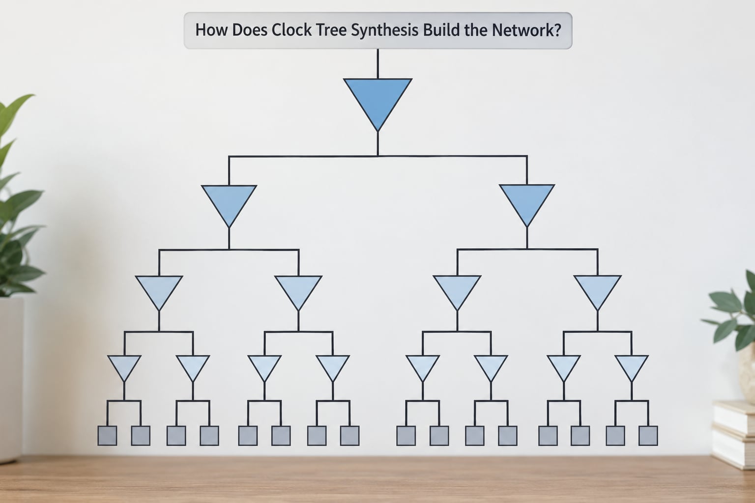
The construction flow runs roughly in this order, and the exact names differ between tools but the stages are the same:

1. Clock definition and root selection. The tool reads create_clock and create_generated_clock objects, recognises which net is the root, and checks that the root cell can drive the total load.
2. Sink extraction. Every clock pin that belongs to the tree is collected and sorted, excluding pins marked as excluded or stopped.
3. Initial propagation. The engine estimates how far each sink is from the root and groups them into levels based on that distance, so sinks at similar range share a level.
4. Balancing. Delay from the root to every sink is equalised, either by adding or removing buffer stages, resizing cells, or moving a tap point. This repeats until every sink sits inside the skew budget.
5. Inversion and gating insertion. Buffers come in pairs and each pair inverts. The tool inserts inverters to control polarity and to place clock gating cells on the branches that need them.
6. Leaf distribution. Final leaf cells are placed near their registers, and any short or over-long connections are cleaned up.
7. Routing and verification. The clock nets are routed, often with wider wires and larger spacing than signal nets, then re-verified with the real extracted parasitics.

Which topologies the algorithms use

Classical papers describe abstract tree shapes; commercial engines use their own hybrid. Knowing the classical ones makes the tool reports easier to read.

Topology	Structure	Skew	Main drawback
H-tree	Symmetric branching from a central point	Near zero by construction	Assumes uniform sink distribution; long and expensive on irregular floors
X-tree	Diagonal branches, like an X	Good on uniform sinks	Non-rectilinear routing, so extra jogs and crosstalk risk
Pi tree	Parallel branches like the Greek letter	Very low on rectangular sink arrays	Poor fit for irregular placement
MMM (Method of Mean and Median)	Groups sinks by geometric centre points	Good, placement-aware	Local optimisation, can leave outliers
GMA (Geometric Matching Algorithm)	Matches sinks geometrically branch by branch	Good	Cost grows with sink count
DME (Deferred Merge Embedding)	Abstract topological merging with real delay merging	What most modern engines lean on	Runtime; needs a good initial clustering

Van Ginneken’s algorithm is the classical reference for the merge-and-embed step that DME builds on: you describe the desired topology abstractly, merge branches downward while respecting the RC delay budget, then embed the result onto the floorplan. That separation is why modern engines can produce excellent skew without ever drawing an H-tree.

What Happens During Clock Tree Synthesis?

Each stage involves a decision, not just an action:

• Balancing — trade minimum skew against total latency. Hitting a very tight skew target often pushes insertion delay up, because the tool pads short branches to match long ones.
• Useful skew — deliberately skewing one register relative to another to buy setup slack. It is a real technique at advanced nodes and it changes what “balanced” means.
• Clock gating integration — gating cells sit inline with the branches they control. Gating placed badly can sit close to the sinks it feeds, and that quietly adds latency to a register group.
• Variation handling — the engine balances across process, voltage and temperature corners, and derates for on-chip variation so the skew that matters is worst-case skew, not nominal.
• Routing rules — clock nets usually get a non-default routing rule: wider wires, larger spacing, sometimes shielding. This protects duty cycle and electromigration but consumes routing resource.
• Post-CTS optimisation — after the first build the engine resizes and re-places cells to recover setup and reduce power without reopening the balance.

One thing worth flagging: the tool makes locally optimal choices against the constraints you gave it. If the constraint is wrong, the local optimum is confidently wrong too.

How Do CTS and STA Work Together?

Static timing analysis and CTS are a two-pass conversation. Before CTS, the clock network is declared ideal: zero insertion delay, zero skew. That models an infinitely fast and perfectly balanced clock, so all reported slack is signal-path slack and setup closure looks optimistic.

After CTS, the tool propagates the real tree. The clock arrival times now differ between registers, and reports gain rows you did not have before: per-register clock latency, local skew, common path versus uncommon path, and a CRPR adjustment applied to the uncommon portion of the launch and capture clock paths.

That shift explains most post-CTS surprises. A path that closed pre-CTS can open post-CTS because the capture clock arrived earlier, tightening hold. A path that failed pre-CTS can improve because the launch clock arrived later.

So the loop is: build the tree, re-run timing with real delays, read the failure attribution, and fix the clock side of the path rather than padding the data path. Interconnect parasitics are estimated during CTS and replaced with extracted values at signoff, so a discrepancy between CTS and post-route reports usually points at routing rules, shielding or an unusually long branch.

How Does CTS Affect Power, Area, and Routing?

The clock network is one of the largest single power consumers in a modern SoC, because every register in a domain toggles on the same edge. Clock power is capacitance times voltage squared times frequency, and the clock tree is large capacitance by construction.

Objective	What it buys	Cost of over-optimizing
Minimum skew	Simpler timing reasoning, cleaner hold behaviour	Higher insertion latency, more buffers, higher peak power, worse congestion
Minimum latency	Shorter clock period available, lower power for a given period	Less room for useful skew, tighter routing
Minimum uncommon path	Less variation derate, more realistic timing	Extra buffering on shared segments
Duty cycle integrity	Reliable high pulses	Wider spacing rules, more routing resource
Signal integrity and EM	No electromigration failures, stable edges	Doubled wire width and spacing, congestion on critical layers
Minimum power	Lower switching capacitance	Fewer, larger buffers; needs a balanced tree to stay safe

The point worth internalising: a perfectly balanced tree is not automatically the smallest or lowest-power design. Pushing skew to its tightest target can add levels to the tree, and every extra level is capacitance that switches every cycle. On some designs a slightly looser skew target gives lower total clock power and easier routing, and that is a legitimate outcome, not a failure.

Clock gating changes the arithmetic substantially. The clock gate ratio — the share of clock cycles a domain is stopped — is reported alongside clock power, and it dwarfs most tree-geometry tweaks. Architecture decisions about gating usually matter more than buffer sizing.

What Problems Can Cause a Bad Clock Tree?

• Excessive skew. Recognise it as post-CTS hold violations clustered on register pairs with very different clock arrival, and as an unbalanced level count across the tree report.
• Unbalanced levels. One branch is much deeper than its neighbours. Visible as a wide spread in the level or distance columns of the CTS report.
• High insertion delay. The whole tree is late, usually because the root cell is too small for the total load or the tree is deeper than necessary.
• Gating placed badly. Back-to-back gating cells, or gating sitting far upstream of the group it controls, add latency silently. Look for unexpected leaf-level cells in the clock structure report.
• Common path dominating. If nearly the whole launch and capture clock path is shared, CRPR removes almost all derate and timing gets optimistic rather than pessimistic.
• Clock tree DRC and EM violations. Spacing, width or electromigration errors on clock nets, usually where the non-default rule was relaxed or the branch runs long.
• Excluded and stopped pins. Pins left out of the tree keep their old RC delay and skew relative to everything else.
• Useful skew gone wrong. Deliberate skew intended to help setup now pushes hold the other way, often only visible after routing.

How Do You Verify and Fix a Clock Tree?

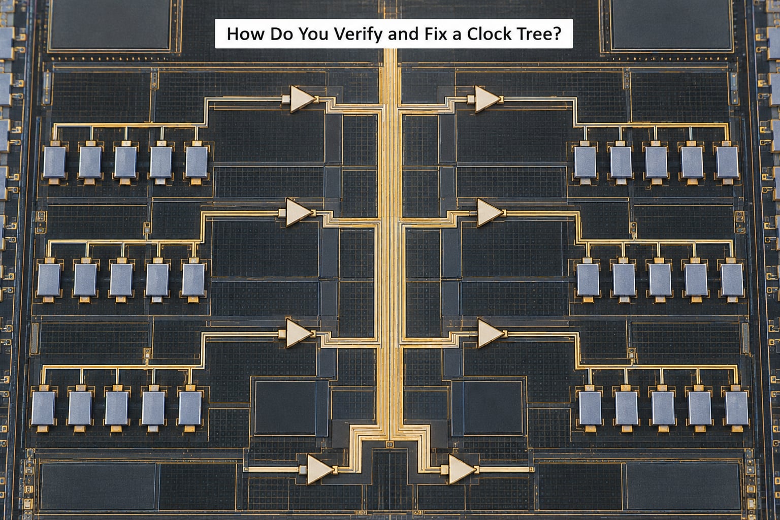
A workable verification pass covers seven things:

1. Pre-CTS timing baseline. With the clock declared ideal, confirm the design closes setup and hold. If it does not, CTS has nothing useful to balance.
2. CTS report. Read total latency, max and mean skew, number of levels, buffer and inverter counts, gating count, and the per-corner spread.
3. Post-CTS timing with real delays. Compare against the pre-CTS baseline and list every path that changed sign or lost margin.
4. Attribution. For each hold failure, split the clock path into common and uncommon portions and check which register pair carries the large uncommon segment. That is the fix target.
5. Power and EM. Check clock power before and after, the gate ratio, and any electromigration or IR drop report on clock nets.
6. Physical checks. Clock DRC errors, spacing on wide clock wires, shielding where the rule requires it, and clock-route congestion.
7. Post-route correlation. Compare CTS estimates against extracted parasitics. A growing gap usually means routing rules were not honoured on a long branch, or a NDR exception leaked in.

Then iterate. Loosen or tighten the skew target, adjust the root buffer, revisit the excluded pin list, or change the clock architecture. Engineers working on this stage describe it as the point where a design either works or does not, and the recurring lesson is that architecture fixes beat tool settings when the tool keeps landing somewhere you did not want.

Clock Tree Synthesis Explained: Key Terms and Design Choices

Term	Meaning	Design choice attached
Insertion delay	Source-to-sink propagation time	Short latency frees clock period but constrains tree depth
Clock skew	Arrival time difference between sinks	Tighter skew costs latency, area and power
Latency	Overall clock delay through the network	Watch it when frequency rises
Useful skew	Deliberate skew used to gain setup slack	Pair it with a hold review of the same registers
Balance level	Tree depth assigned to a sink	Uneven levels point at a placement or root problem
Clock cell	Buffer, inverter or gating cell in the tree	Choose drive and footprint deliberately, they set power
OCV / AOCV / POCV	On-chip variation derating models	Drives how much skew budget you actually need
CRPR	Common path pessimism removal	Check the common portion is genuinely common
ECO	Engineering change order after CTS	Local tree changes need a full re-verification pass

Frequently Asked Questions

Conclusion

Clock tree synthesis explained comes down to one idea: a single clock port cannot drive a die’s registers directly, so the tool builds a buffered, balanced network that delivers every edge at nearly the same moment, at an acceptable cost in latency, area and power.

Start by getting the clock intent right — the SDC spec, the excluded pins, the skew target and the gating structure. Everything after that, including post-CTS skew, latency, power and the physical checks, is easier to reason about once the constraints match the architecture. Update this guide for 2026: the fundamentals have not moved, but derating models and clock routing rules on the newest nodes keep changing.