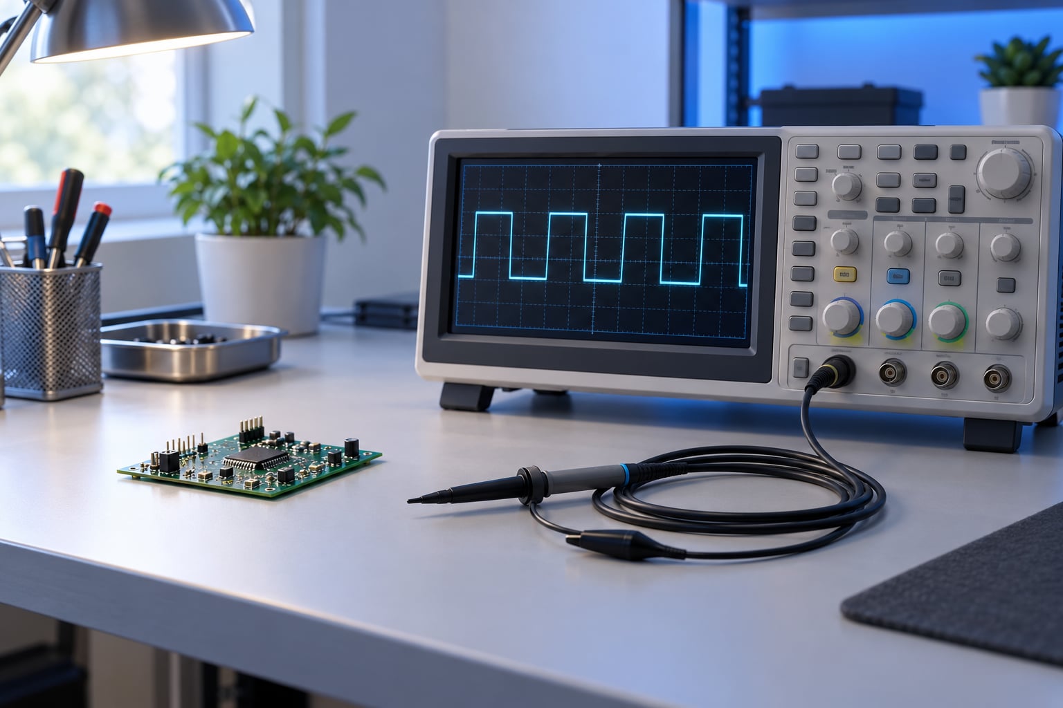
To use an oscilloscope for digital signals, you connect a probe to the logic-level net, set the probe attenuation to 10X, scale the trace to a few divisions tall with DC coupling, and trigger on a rising edge so the display stops scrolling. Once the waveform stands still, you read voltage and timing off the cursors and compare the numbers against the datasheet limits for that net. A competent setup takes about ten minutes, and the hardest part for beginners is grounding, not the knobs.
Most first-week confusion comes from one thing: a digital signal is an analog waveform that just happens to be interpreted as a one or a zero. The scope shows you the real volts and the real microseconds, which is exactly what a logic analyzer throws away. That is why engineers reach for the scope first when a bus misbehaves.
Table of Contents
- What You Need
- The safety rules that matter
- Step-by-Step
- How to Use an Oscilloscope for Digital Signals
- Set the Vertical and Horizontal Controls
- Trigger the Signal Correctly
- Measure Voltage, Timing, and Logic Levels
- Interpret Common Digital Waveforms
- Verify and Save the Measurement
- Common Mistakes
- Frequently Asked Questions
- What probe should I use for digital signals?
- How do I set an oscilloscope to trigger on a digital signal?
- What oscilloscope bandwidth is needed for my digital circuit?
- Why does my digital waveform look unstable on the oscilloscope?
- Can an oscilloscope measure UART, I2C, or SPI signals?
- How do I tell if a digital signal has too much ringing or overshoot?
- Conclusion
What You Need
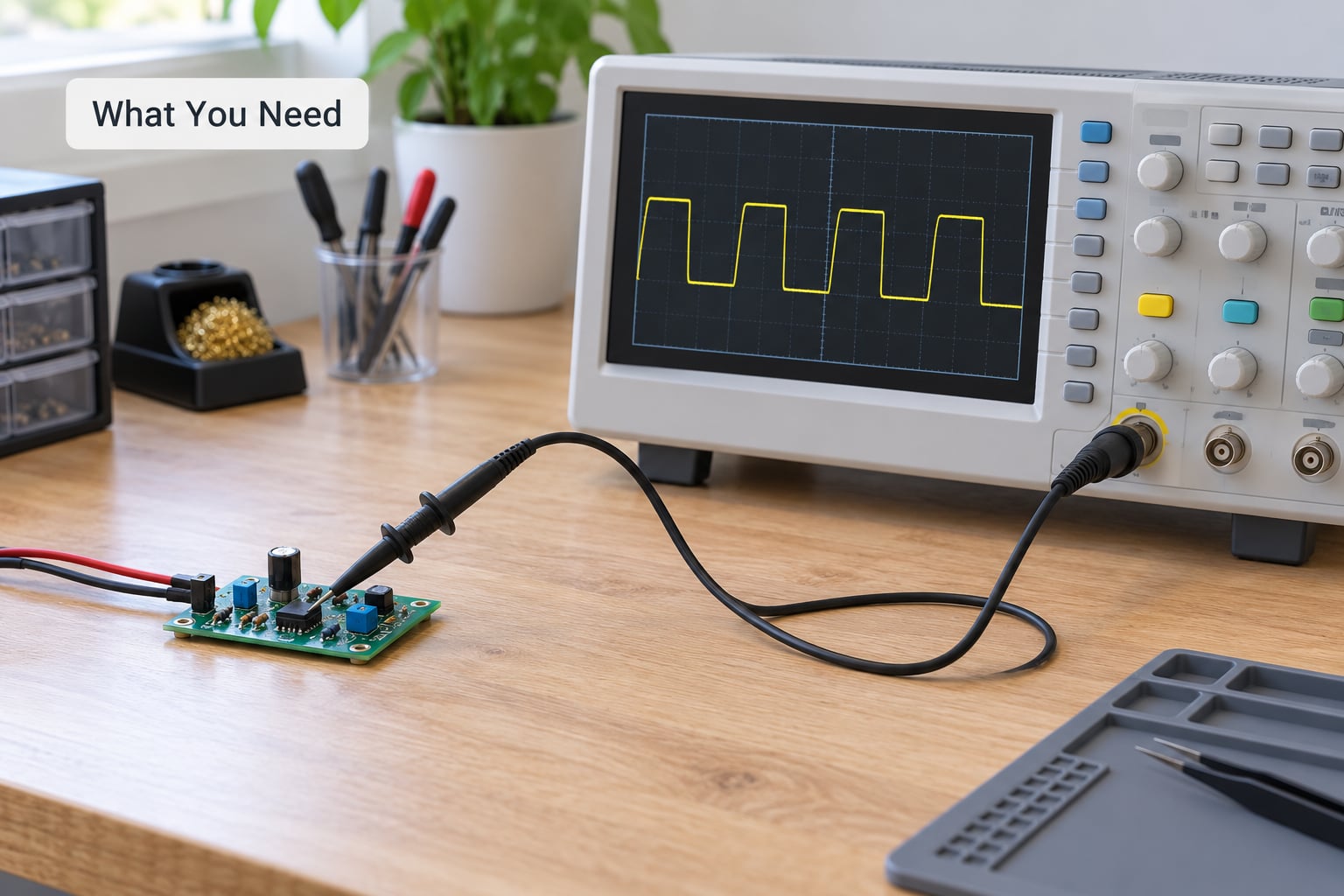
You need four things, and only one of them is expensive.
- An oscilloscope with at least two analog channels. A digital storage oscilloscope (DSO) is enough. A mixed-signal oscilloscope (MSO) adds threshold-reference digital channels, which is useful later but not required to start.
- A 10X passive probe per channel. Standard probes add roughly 10 to 15 pF of input capacitance and present about 10 megohms of input impedance. Every probe needs its own ground connection, even when the grounds are common inside the scope.
- A ground spring or a short ground lead. The clip leads that ship with probes often run 6 inches or more of wire, which is the single largest source of bad measurements.
- A device under test with accessible test points. If you have to solder a wire to a fine-pitch pad to probe it, you will be back on the bench with a different board next time.
Add the reference documents before you power anything up: the device datasheet for voltage and timing limits, and the schematic for the net name. The scope is the measuring tool, not the specification.
The safety rules that matter
Oscilloscope inputs are generally rated to earth ground through the probe, and the probe tip is shorted to the ground lead internally. Clip that ground lead to a live node and you have put a mains-referenced short across your circuit.
Three rules cover almost every bench accident I have seen: clip the ground to system ground only, power the circuit down before moving the ground clip, and never probe a mains or high-voltage node with a grounded scope. For floating or high-side nodes, use a differential probe or a battery-powered scope. Checking with a multimeter before you clip is cheap insurance against soldering a damaged board back together.
Step-by-Step
This is the repeatable workflow. Follow it in the same order every time and most beginner problems disappear on their own.
How to Use an Oscilloscope for Digital Signals
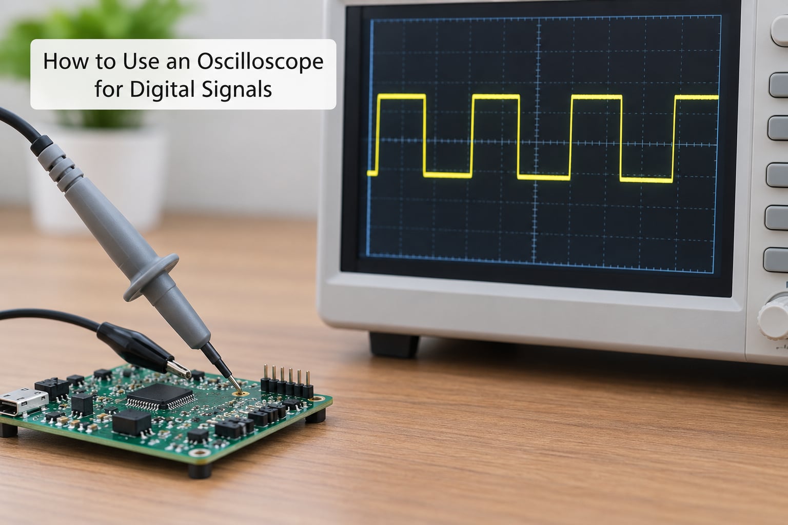
The core process has six moves: connect the probe, select the channel, set probe attenuation, choose voltage and time scales, establish a stable trigger, then verify against expected logic levels and timing. Do the trigger step last, because until the vertical and horizontal scales are right, a stable display means nothing.
| Task | What you do | How you know it worked |
|---|---|---|
| Power and ground | Power the board, then attach the probe ground spring to system ground near the probe point | The board stays powered and the rail reads its nominal voltage with cursors |
| Connect the probe | Tip on the net, ground spring on the reference point, no other clips attached | A flat line or a plausible square wave, not a wildly drifting trace |
| Set attenuation | 10X on the scope channel to match the 10X probe | The amplitude on screen matches the expected logic swing |
| Set coupling and scale | DC coupling, about 1 V per division, 100 us to 1 ms per division for a first look | Two to four divisions of peak-to-peak swing, two to four cycles across the screen |
| Trigger | Source on that channel, rising edge, level near the mid-point of the swing | The trace stops scrolling and the same waveform sits still |
| Measure | Turn on automatic measurements, then confirm the key values with cursors | Period and pulse width repeat with no jitter beyond expectation |
Set the Vertical and Horizontal Controls
Channel coupling decides what reaches the screen. DC coupling passes the whole signal, so a 3.3 V rail shows as 3.3 V and any droop on the net is visible. AC coupling blocks the DC component, which is correct for looking at ripple on a supply but wrong for logic levels, because it hides where the low actually sits.
Probe attenuation multiplies what the scope displays. A 10X probe divides the input by ten before display, so the scope must be set to 10X or every reading comes out ten times too high. If the trace looks like it has far more amplitude than the circuit can produce, the first thing to check is this setting on both the probe body and the channel menu.
Volts per division sets the height of the trace. Start near the expected swing so a 3.3 V signal fills about three or four divisions, which leaves headroom to see overshoot. Offset shifts the trace vertically without changing the scale, which is how you move a second signal to a clear part of the screen. If a trace runs off the top or bottom of the display, the amplifier is clipping and every measurement from that channel is invalid; reduce volts per division or fix the offset first.
The time base controls seconds per division. For a clock, set the horizontal scale so two to four cycles span the ten divisions, then zoom in for detail. Peak detect acquisition catches narrow glitches that a slower sample rate would otherwise skip, averaging cleans up random noise on a repetitive signal, and single-shot acquisition captures one event for signals that do not repeat, such as a reset assertion at power-up.
Trigger the Signal Correctly
The trigger is what makes a digital waveform readable. It tells the scope the exact instant to start each sweep, so repeating edges land in the same place every time. Set the trigger source to the channel you are probing, choose a rising edge, and set the level to roughly the mid-point between the low and high levels of your signal.
Three trigger modes cover most work. Auto mode sweeps whether or not a trigger event occurs, which is why an untriggered trace in auto looks like it is scrolling rather than standing still. Normal mode waits for a real event, so an untriggered display simply freezes. Single mode fires once and holds the capture, which is what you want for a pulse that arrives only after a command.
Beyond edge triggers, most scopes offer a few that map directly onto digital failures. A runt pulse trigger captures edges that are too narrow to be a valid bit. A glitch or pulse-width trigger fires only when a pulse falls outside a time window you set, which is how you catch a single-corrupted-edge condition in a long frame. A window trigger fires only when the signal is inside a voltage and time box, useful for isolating a specific state in a repeating sequence. Trigger holdoff blanks the sweep for a set time after each trigger, which stops the display from locking onto the wrong edge in multi-cycle patterns such as a divided clock or a burst.
If the waveform still will not stand still, work down this list: move the trigger level closer to the mid-swing, switch from AC to DC trigger coupling, change source from the main clock to the data line, or add holdoff equal to roughly one period of the repeating pattern.
Measure Voltage, Timing, and Logic Levels
Automatic measurements give you numbers fast, cursors give you numbers you can trust. Use both, and cross-check the two values that matter most for the device under test.
| Measurement | How to make it | What a healthy value looks like |
|---|---|---|
| High and low level | Cursors on the flat top and flat bottom, or Vhigh and Vlow automatic measurements | Output high (VOH) and output low (VOL) both inside the datasheet limits |
| Peak-to-peak swing | Vpp cursors from the top rail to the bottom rail | Close to the supply rail for an unloaded CMOS output |
| Period and frequency | Automatic frequency, confirmed with two time cursors on adjacent edges | Frequency matches the oscillator or datasheet nominal |
| Pulse width and duty cycle | Positive pulse width cursors on a rising and a falling edge | Stable across many cycles, within the timing budget of the design |
| Rise and fall time | Cursor from the 10 percent level to the 90 percent level on the same edge | Fast enough for the receiver, and slow enough to avoid ringing |
| Input thresholds | Compare measured crossing points against input high voltage (VIH) and input low voltage (VIL) | Every valid crossing passes cleanly through the input threshold window |
For timing relationships between two signals, put each on its own channel and use cursors across channels, or use two cursors in a delta mode. That is how you check setup and hold time on a data bus, propagation delay between a strobe and its data, or the delay from command to acknowledge on a serial bus.
Keep the bandwidth limit filter in mind. Turning it on at 20 MHz removes high-frequency noise from the trace and stops ringing from dominating the edge measurement, but it also makes the rise time look longer than the net really is. Know which state you are in before you report an edge rate.
Interpret Common Digital Waveforms
Clean digital logic looks almost boring: flat tops, flat bottoms, vertical edges, and a steady period. Everything else tells you something about the circuit.
Ringing shows as decaying oscillation right after an edge. It means the edge is fast enough to excite the trace capacitance against the line inductance, usually combined with a mismatch between driver output impedance and trace impedance. A little ring is normal on a fast edge. Heavy ring that crosses back below the receiving threshold risks a false transition, and the fix is damping at the source, not a slower probe.
Overshoot and undershoot are excursions above the high rail or below the low rail on a transition. Small amounts are expected from the edge rate. Large excursions can damage a device that specifies an absolute maximum supply range, so treat them as a defect rather than a curiosity.
Droop or a sagging rail appears as the low level of a signal slowly sliding downward, usually on a heavily loaded net or during a switching event. A drooping rail reduces noise margin, and the digital logic still works until it does not.
Missing pulses or narrow runt pulses appear as a trace that is fine except for one thin spike. In peak detect or single-shot mode, widen the time base until you can see what the spike is, then trigger the runt or glitch detector to capture it. Many of these are coupling from a switching node on the board, not real logic activity, and moving the probe point a few millimetres often makes them vanish.
Noisy tops and bottoms mean the voltage is not settled. Either the drive is too weak for the capacitance, the threshold is not being met, or your ground reference is moving. Check the ground spring before you start blaming the circuit.
Verify and Save the Measurement
A measurement you cannot repeat is an anecdote. Confirm the key values at least twice, on separate captures, and check that they agree.
Compare each number against the specification. A clock at 100.02 MHz is fine if the tolerance is one percent, and a problem if the tolerance is 0.1 percent. A 0.4 V high level against a 0.8 V minimum is a fault regardless of how clean the trace looks.
Write down three things with every capture: the probe point, the probe attenuation and coupling, and the vertical and horizontal scale. Then save a screenshot with those settings visible on the display if you can. When the failure comes back in two weeks, that record is the difference between a five-minute diagnosis and an afternoon of guessing.
For a repeatable production or validation setup, script the measurement sequence. Automated test equipment on a probe card does exactly this workflow, one channel and one timing parameter at a time, and produces the same record every run.
Common Mistakes
Probe attenuation set wrong. A 10X probe with the scope on 1X shows every amplitude ten times too high. Set 10X on both the probe body and the channel, and confirm with the scope’s own probe compensation output.
Ground clip on the wrong node. This is the most common cause of corrupted readings and it is the one beginners hit hardest. Clip to system ground on the same board, as close to the probe point as you can reach. Clipping to a different ground point forces current from your circuit through the probe ground wire, and that added resistance turns millivolts of ground difference into tens or hundreds of millivolts of offset in your reading. A common community diagnostic is to touch the probe tip directly to the ground clip, shorting the input. If the noise on your trace disappears, the problem is your reference point, not the circuit.
Long ground leads on fast edges. A six-inch ground lead is an antenna and an inductor. Swap it for a ground spring, or twist the lead down to a few millimeters. This one change fixes more noisy traces than any setting on the scope.
Wrong input coupling. AC coupling on a logic signal hides the actual low level, so a signal that fails the input low voltage (VIL) limit can look acceptable. Default to DC coupling for digital work and use AC only for ripple and small-signal overlay.
Unstable triggering. A scrolling trace usually means auto mode with no trigger event, a trigger level set above or below the swing, or a source pointing at the wrong channel. Complex repeating patterns need holdoff. Patterns that never repeat at all need single-shot.
Not enough bandwidth. A common rule of thumb is that the scope bandwidth should be several times the signal frequency so you can see the first several harmonics that shape an edge. A 100 MHz scope on a 100 MHz clock shows a rounded blob; 500 MHz shows a recognisable edge. Remember that probe and input capacitance also limits how fast an edge you can see, and a fast probe on a slow source can ring.
Ignoring probe loading. A 10X probe adds roughly 10 to 15 pF to the node. On a slow net that is invisible. On a short net with a fast edge, the probe can slow the edge down and change the very thing you were trying to measure. Check with a second channel when the answer matters, or use a low-capacitance active probe.
Confusing the ground clip with a signal connection. The probe is coaxial. The tip is the signal input, the ground lead is the reference, and there is no third connection. If a floating probe tip shows a voltage, that is capacitive pickup from whatever is nearby, not a real reading.
Two habits close most of these. Calibrate the probe on the scope’s 1 kHz calibration output before each session: a flat top with sharp corners is correct, rounded edges mean under-compensation, and a pointed overshoot at the top means over-compensation. And power down before moving ground clips, every time.
Frequently Asked Questions
What probe should I use for digital signals?
Use a 10X passive probe for almost all digital work below about 100 MHz. It protects the scope, and its roughly 10 megohm input impedance and 10 to 15 pF capacitance load the net lightly. Set the scope channel to 10X to match, and use a ground spring instead of the clip lead. Above that, step up to a low-capacitance active probe, and use a differential probe whenever the node is floating, high-side, or the two ends of your measurement sit at different potentials.
How do I set an oscilloscope to trigger on a digital signal?
Set the trigger source to the channel carrying the signal, select a rising edge, and set the level to the mid-point between the signal’s low and high levels. Use normal mode rather than auto so the display holds still, and switch to single-shot for a one-time event. If a repeating multi-cycle pattern keeps showing different cycles, add holdoff of roughly one period. If the trace is still noisy, move the level closer to the mid-swing and use DC trigger coupling.
What oscilloscope bandwidth is needed for my digital circuit?
Pick a bandwidth several times your clock frequency, roughly three to five times, so the edge is resolved rather than rendered as a rounded blob. A 100 MHz scope on a 100 MHz clock is barely usable; 500 MHz shows the edge clearly. Remember that bandwidth alone is not the whole story: probe capacitance slows fast edges, the sample rate and memory depth decide whether you capture narrow glitches, and the waveform update rate decides whether a rare fault is ever displayed.
Why does my digital waveform look unstable on the oscilloscope?
Four causes account for nearly every unstable trace. The trigger is in auto mode with no event occurring, so the sweep free-runs. The trigger level sits above or below the signal swing, so no edge ever matches it. The ground clip is on a different ground point than the circuit, injecting offset. Or a repeating pattern needs holdoff so the scope stops locking onto the wrong edge. Check the trigger settings first, then swap the clip lead for a ground spring.
Can an oscilloscope measure UART, I2C, or SPI signals?
Yes. A scope with protocol decoding can trigger on and decode UART, I2C, and SPI, and most mixed-signal oscilloscopes support CAN and LIN as well. The decode gives you bytes and frames; the scope waveform still gives you rise time, overshoot, ringing, and timing violations that a decoder hides. Many people use both together. A logic analyzer captures long sequences more cheaply, while the scope is the better tool for the analog quality of a single edge.
How do I tell if a digital signal has too much ringing or overshoot?
Look at the first cycle after a fast edge. Decaying oscillation that crosses back through the receiving input threshold is real ring, and it can register as a false transition, so treat it as a failure. Excursions above the high rail or below the low rail are overshoot and undershoot; small amounts are normal for a fast edge, but large ones can exceed a device absolute maximum supply rating. Fix the cause with source termination or a series damping resistor rather than by slowing the probe.
Conclusion
Start every session the same way. Identify the net and find its specification, connect the probe with a ground spring on system ground, set 10X attenuation and DC coupling, scale the trace to a few divisions with two to four cycles visible, then trigger on a rising edge at the mid-swing. Measure, compare against the datasheet, and record the probe point and settings with the capture.
Most disappointing results trace back to grounding rather than to the instrument. Get that right and the rest of learning how to use an oscilloscope for digital signals gets much faster.