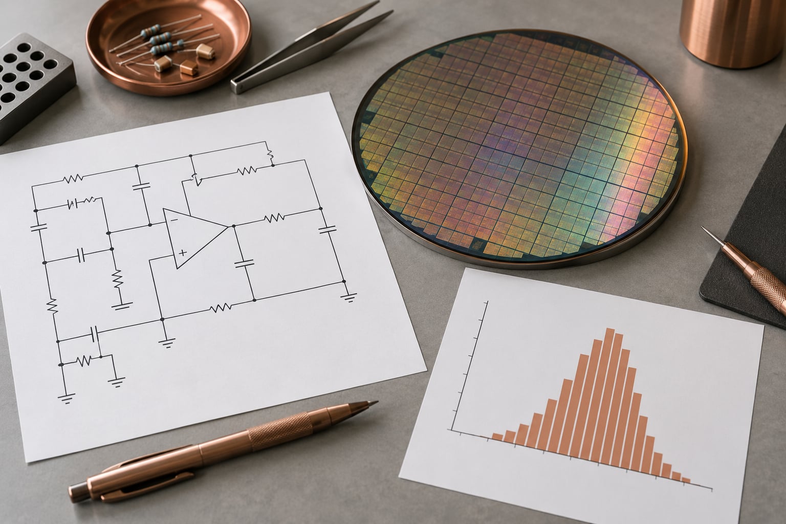
Monte Carlo Simulation in Analog Design Explained 2026

Monte Carlo simulation in analog design explained, in one line: it runs your circuit hundreds or thousands of times while randomly varying process, mismatch and component values, then shows you the distribution of results instead of a handful of corner points. That distribution is what tells you whether a design will hold up across a million parts, not just across the four corners you typed in last week.

The rest of this article goes step by step, from where variation comes from, through how the sampling actually works, to how many runs you can afford and how to read what comes back.

Table of Contents

• What Monte Carlo Simulation in Analog Design Does
• Why Real Circuits Are Not Identical
• How Monte Carlo Analysis Works in an Analog Circuit
• A worked example: Monte Carlo simulation on a current mirror
• Choosing Inputs, Distributions, and Statistical Models
• Reading Yield, Failure Probability, and Performance Spread
• Monte Carlo Simulation Versus Process Corners
• A Practical Example for an Operational Amplifier
• How to Reduce Simulation Time Without Losing Confidence
• Common Mistakes and Misinterpretations
• Frequently Asked Questions
• How many Monte Carlo runs should an analog designer use?
• Is Monte Carlo simulation required if I already run process corners?
• What is the difference between process variation and mismatch?
• How do I calculate yield from Monte Carlo results?
• Which analog measurements should I monitor during a statistical run?
• Can a language model run a Monte Carlo simulation for my circuit?

What Monte Carlo Simulation in Analog Design Does

Monte Carlo simulation in analog design is a statistical analysis method. The simulator repeatedly solves your circuit while drawing device and component parameters from their characterised distributions, then records a measurement such as gain, offset voltage or passband ripple for each run. The result is a population of outcomes, and the fraction that meet your specification is the predicted yield.

That is the whole difference from other flows. A nominal run tells you what happens at the numbers on your schematic. A corner run tells you what happens at deliberately chosen extremes. A Monte Carlo run tells you what happens in a factory, where nothing sits at an extreme but everything drifts a little.

It is also the only one of the three that captures random mismatch, the device-to-device scatter inside a single die that corner analysis cannot represent at all, because two nominally identical transistors on the same piece of silicon simply are not identical.

Why Real Circuits Are Not Identical

Nothing comes out of a fab exactly as drawn. Global variation moves a whole die or a whole wafer in the same direction, so every resistor on the die is 1 percent high together. Local variation, usually called mismatch, moves each device independently, so two adjacent transistors can land anywhere within their tolerance bands at the same time.

Add supply voltage drift, ambient temperature, load impedance and the tolerance of every external resistor, and the number of combinations a real part experiences is astronomically larger than the number of corner boxes you have in your test plan.

This distinction matters more than it sounds. Global variation shifts the operating point of the whole circuit and mostly behaves like a slow corner sweep. Mismatch breaks symmetry inside the circuit, and symmetry is what offset voltage, current mirror ratio accuracy and common-mode rejection depend on.

Variation type	Scope	What moves together	Design lever
Global, wafer-to-wafer	One value per wafer or lot	Every device of the same type on the die	Process corner sweeps, guard bands
Global, die-to-die	One value per die	Every device of the same type on that die	Corner sweeps, trimming, calibration
Local variation, mismatch	One value per device	Nothing, by definition	Common-centroid layout, larger devices, chopping, trimming
Passive tolerance	Per component	Nothing unless correlated by design	Tighter parts, calibration, ratioed trimming
Environment	Per part in the field	Often correlated with board conditions	Headroom, regulation loop, thermal design

How Monte Carlo Analysis Works in an Analog Circuit

The mechanism is straightforward once you see that it is just a loop. Everything else in this article is detail on one of these six steps.

1. Define the parameters. Pick which inputs will vary. In an IC flow these usually come straight from the PDK statistical models: threshold voltage, effective channel length, oxide thickness, mobility, gate oxide capacitance and doping.
2. Assign distributions. Most PDK parameters ship with a statistical model already attached, often a Gaussian or a Pelgrom-style mismatch model. Discrete resistors and capacitors get tolerance distributions from their datasheets.
3. Set the run count. Choose how many trials, and whether the run is process-only, mismatch-only, or both together.
4. Simulate. The simulator solves the testbench repeatedly and stores each result in a results database.
5. Measure. For every run, record the numbers you care about, using assertions or measurement expressions in the testbench.
6. Post-process. Build histograms, compute pass rates, and look at the tails rather than the average.

As an illustration, take a gain measurement. Draw 500 runs, plot them, and the mean tells you almost nothing useful. What matters is the spread, and whether the distribution has a shoulder that crosses your lower gain limit at 3.5 percent of runs. That 3.5 percent is your real answer: about 3.5 percent of parts fail the gain spec.

A worked example: Monte Carlo simulation on a current mirror

A 1:2 current mirror is the classic teaching case because the arithmetic is simple and the failure mode is invisible in simulation until you look for it. Both devices have the same nominal overdrive set by a bias current, so nominally the ratio is 1:2 exactly.

Add mismatch and the two transistors have different threshold voltages and different effective channel lengths, so the ratio scatters. Halve the area of both devices and the Pelgrom mismatch coefficient makes the relative scatter grow roughly in proportion to the inverse square root of device area, which is why small current mirrors fail in production while large ones do not.

Run 500 trials, measure the ratio on each, and the histogram is a clean bell curve centred on 2.0. A specification of 1.95 to 2.05 may look generous until you notice that the standard deviation is 0.04, which puts 4 percent of parts outside the window. A pure corner sweep would have shown you a single clean 2.0 and told you nothing at all.

Choosing Inputs, Distributions, and Statistical Models

Choosing what to randomise is where most first attempts go wrong. The rule of thumb is that anything that varies in production and affects your measurement belongs in the run, and nothing else does.

Parameter	Variation type	Typical distribution	Usual treatment
Threshold voltage Vth	Global and local	Gaussian via PDK model	Always randomise
Effective channel length	Global and local	Gaussian, right-skewed	Always randomise
Mobility and Tox	Global, strongly correlated	PDK model, correlated	Randomise with Vth, keep correlation
Device mismatch	Local, per device	Pelgrom area law	Separate mismatch-only run
Resistor or capacitor value	Per component	Uniform or triangular across tolerance	Only if outside silicon
Supply voltage	Environmental	Uniform over the specified range	Separate run, not mixed with process
Temperature	Environmental	Discrete cases	Keep as corners, not random

Uniform and triangular distributions suit datasheet tolerances, because all you know is a bound and no more. Gaussian is right for process parameters where a foundry has characterised a mean and a spread. A correlation-aware model beats five independent Gaussians every time, because mobility, threshold voltage and oxide thickness move together on a real wafer and pretending otherwise widens your distributions artificially.

Tie your parameter spread to something real. If you set Vth sigma to an arbitrary number, your yield estimate is fiction. The PDK statistical models, and the wafer probe data that calibrates them, are the only defensible source.

Reading Yield, Failure Probability, and Performance Spread

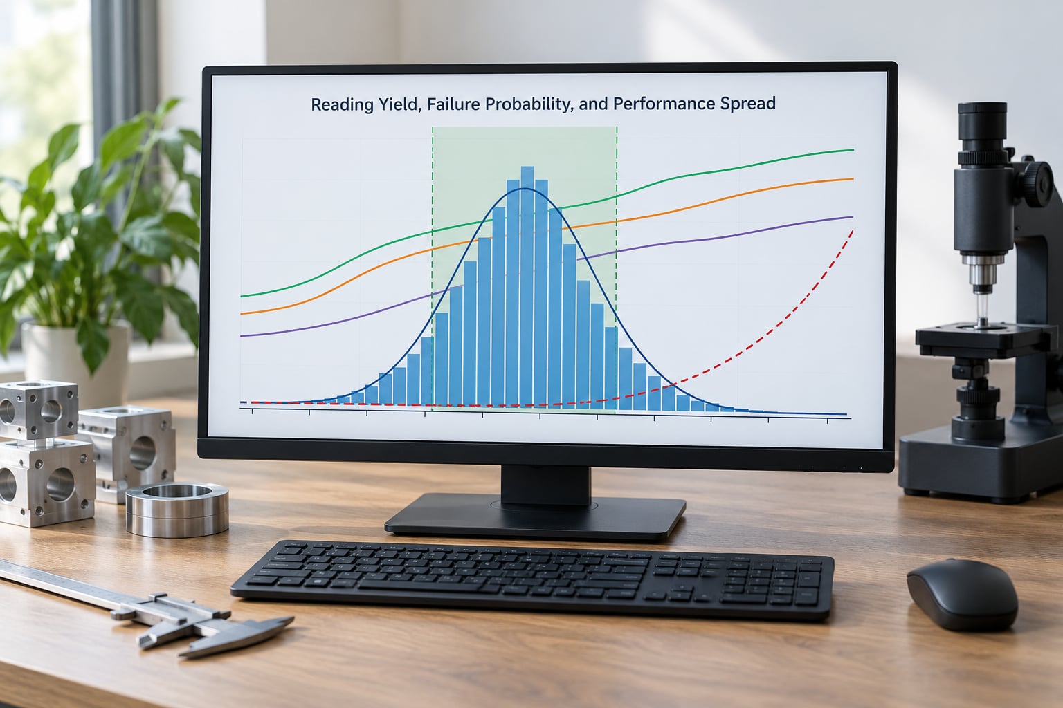
Read the histogram, not the average. The habit most worth breaking early is averaging the output, because a distribution averaged to a single number tells you nothing about the parts that fail at the edges. Monte Carlo runs exist to show how bad performance can get, and the worst case is rarely where every parameter sits at its tolerance limit together.

Three numbers carry most of the meaning. The pass rate is the fraction of runs inside your assertion limits, and it is your yield estimate. The capability index compares your spread against the width of the specification window, and a value near 1.0 means you are already producing fallout with no margin left for modelling error.

The third is the tail. Most histograms look healthy in the middle and fail quietly at 3.5 sigma. Sort your failing runs and look at what they have in common. Failures cluster, and clusters point at a mechanism, usually a specific parameter rather than a general lack of margin.

Keep a margin deliberately. A design that simulates at 99.5 percent yield on a model you trust will not hold that number on silicon, because the model, the layout and the packaging all add variation you did not simulate.

Monte Carlo Simulation Versus Process Corners

Corners and Monte Carlo answer different questions, and the useful move is to run both. Corners ask whether the circuit survives deliberately chosen extremes. Monte Carlo asks what fraction of real parts meet spec, and what the distribution looks like along the way.

Aspect	Corner analysis	Monte Carlo analysis
Question answered	Does it survive the extremes I picked?	What fraction of parts pass, and why do some fail?
Inputs	Named PVT corners	Distributions over many parameters
Simulation count	Typically 4 to 20	Hundreds to hundreds of thousands
Output	Pass or fail per corner	Distribution, yield, Cpk, failure modes
Device mismatch	Not represented	Captured directly
Worst case	Unrealistic combination, so often too pessimistic	Realistic, so often too optimistic if run count is low
Runtime cost	Minutes	Hours to days, scaling with run count
Best use	Fast sanity check during design entry	Yield prediction and design-margin sizing

The combination works like this: corners clear the obvious failure modes cheaply, then Monte Carlo finds the combinations nobody thought to type into a corner box. Environment variation is usually kept separate again, as deterministic cases, because supply and temperature drift are not random from one die to the next within a wafer.

A Practical Example for an Operational Amplifier

An op amp makes the method concrete because a handful of measurements tells you whether the architecture works, and each measurement exposes a different weakness.

Randomise the process parameters and device mismatch, keep supply and temperature fixed, and collect open-loop gain, unity-gain bandwidth, output offset, output swing and the phase margin you get from the loop gain. Run a few hundred trials and plot each measurement.

Offset voltage is the first to look bad, because it is dominated by mismatch between the input pair and it scales with the inverse square root of input device area. Gain spreads more gently and is mostly a global process effect. Output swing tells you whether your cascode headroom survives a slow, high-threshold corner, and phase margin is where the tail hides, because a few samples cross into instability while the histogram still looks respectable.

The design response follows directly. Increase input device area to pull offset in, add a cascode or more headroom for the swing failures, and if phase margin is the problem, add compensation capacitance rather than increasing bias current. Trim or chop if offset alone is out of reach.

Then carry the same numbers into layout. A Monte Carlo run that randomises mismatch but ignores placement will understate offset badly, because devices placed in a common-centroid layout cancel far more mismatch than the statistical model assumes for random placement.

How to Reduce Simulation Time Without Losing Confidence

Runtime is the real objection to large Monte Carlo campaigns, and it scales directly with the number of runs. A few habits cut the cost without weakening the result.

• Separate global and local runs. Process and mismatch contribute differently to different measurements, so run them apart and combine the results statistically when you need the joint picture.
• Start with a screening pass. One or two hundred runs take minutes and will show you which measurements are even at risk. Escalate only the ones that fail.
• Measure less. Every saved measurement costs post-processing time across thousands of runs. Keep the ones tied to a specification.
• Reuse corner knowledge. If a parameter is already pinned by a corner sweep, hold it fixed in the statistical run.
• Use lower-accuracy solver settings for screening. Relax tolerances for the screening pass and tighten them for the final sign-off run.
• Use stratified or quasi-random sampling. These fill the parameter space far more evenly than pure random sampling, so you get a usable answer at a fraction of the runs.
• Use high-sigma methods for the tail. If you need a confidence statement at 5 or 6 sigma, dedicated high-sigma sampling reaches that region far more cheaply than brute-force runs.
• Parallelise. Almost every commercial simulator will shard a Monte Carlo sweep across cores or a farm, and this is usually the single biggest speedup available.

A quick screening run of 200 samples is plenty to catch a design that is badly broken. It is nowhere near enough for a tail claim, because at 1 percent yield you have seen roughly two failures and cannot say anything reliable about how rare the worst case really is.

Common Mistakes and Misinterpretations

Most disappointing Monte Carlo results come from setup problems rather than from the circuit.

1. Averaging the output. This is the most common misunderstanding. The average of a distribution tells you nothing about the parts that fail.
2. Confusing process variation with mismatch. Global variation moves everything together; mismatch moves devices independently. Running one without the other gives an optimistic offset estimate.
3. Treating correlated parameters as independent. Mobility, threshold voltage and oxide thickness are correlated, and splitting them apart widens the simulated spread beyond reality.
4. Randomising convenient variables only. If the specification cares about offset, randomising supply voltage and temperature tells you nothing about offset.
5. Inventing parameter spreads. An arbitrary sigma produces an arbitrary yield number. Use the PDK model.
6. Reporting yield without the run count. Zero failures in 200 runs is a 95 percent upper bound near 98 percent yield, not a 100 percent yield claim. Give the count with the number.
7. Mixing process, supply and temperature into one run. They behave differently and combining them makes the result impossible to interpret.
8. Treating simulation as proof. Monte Carlo is statistical evidence about your models. It does not bound what it has not sampled, and it cannot tell you that no combination exists outside your run count.
9. Ignoring layout when simulating mismatch. Real layouts cancel more mismatch than the statistical model assumes, and badly drawn layouts cancel far less.
10. Stopping when the histogram looks fine. The tails are the part you have not sampled yet.

Frequently Asked Questions

If you do one thing first, add a 300-run process-plus-mismatch campaign to a circuit you already believe in, plot the pass rate for your real specification limit, and read the failing samples. That single exercise usually tells you more about your design margin than another week of corner sweeps.